Age Frameworks

Bouafia Imène

This Vignette introduces the tools in BayLumPlus that extend the original framework for age modelling.

library(BayLumPlus)
#> Loading required package: coda

Age Models Function

In this section we present the splitting of the OSL Model presented in Combès and Philippe (2017). We summarize our approach in the following hierarchical model:

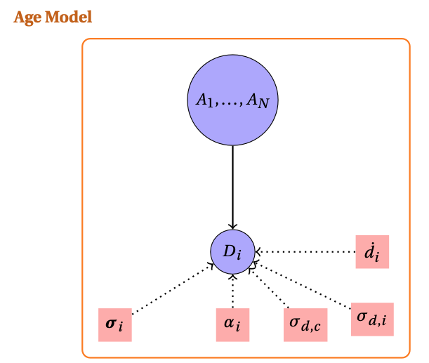
The model incorporates three primary data vectors:

• $\mathbf{A} = (A_1, \ldots, A_n)$: the unknown ages to be estimated.
• $\mathbf{D} = (D_1, \ldots, D_n)$: the equivalent doses obtained from luminescence measurements.
• $\boldsymbol{\sigma} = (\sigma_{1}, \ldots, \sigma_{n})$: the measurement uncertainties for equivalent doses.

The environmental context is characterized by known parameters:

• $\boldsymbol{d} = (d_1, \ldots, d_n)$: mean annual dose rates for each sample.
• $\boldsymbol{\sigma}_{d} = (\sigma_{d_1}, \ldots, \sigma_{d_n})$: individual dose rate uncertainties.
• $\boldsymbol{\alpha} = (\alpha_1, \ldots, \alpha_n)$: contamination factors relating to systematic uncertainty.

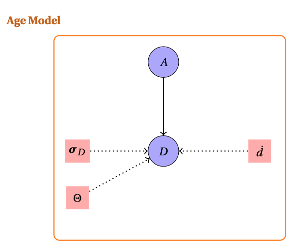
However, this approach does not allow us to account for the complex modeling of common errors. Therefore, instead of considering one common error and a contamination factor, we set the $\Theta$ matrix which represents the covariance matrix that summarizes the several common errors we can consider (see documentation of create_ThetaMatrix()).

The considered model can be summarized by the likelihood:

$$D \sim \mathcal{N}\left( \text{diag}(A) \boldsymbol{d}; \ \text{diag}(A) \Theta \text{diag}(A) + \text{diag}(\boldsymbol{\sigma}) \right)$$

The function allowing to compute such configuration is Compute_AgeS_D().

In the following sections, we demonstrate how to use this function with practical examples.

Measurements quantities

The function needs parameters (see ?Compute_AgeS_D() ) such as a list of DATA composed of
- Equivalent Doses: $D$
- Dose rate: $d$
- Standard Error for $D$: $\boldsymbol{\sigma}$

An example of what it might look like

DATA = list( D = Doses, 
             ddot = dose_rate, 
             sD = standard_error_D)

Stratigraphics prior knowledge

The function can also require a matrix that summarizes the stratigraphic constraints called StratiConstraints. Multiple choice are accepted :
- A numeric matrix such as in create_ThetaMatrix() (meaning with a row of ones)
- A path to a csv file

Note that several prior distributions can be tested:

• Without stratigraphic constraints:
  • unconstrained_Jeffrey
• Under strict order: $\lbrace A_1 \leq \cdots, \leq A_n \rbrace$
  • StrictNicholls&Jones : Nicholls & Jones applied directly to ages (see section 4 in Nicholls and Jones (2001) )
  • constrained_Jeffrey : Approached Jeffreys form

For more information use help(ModelAgePrior).

For these priors there is no need to specify the parameter StratiConstraints as it is supposed to be the strict order or no constraints at all.

You can use the extract_Jags_model() function to check all available models and data structures in BayLumPlus.

To illustrate usage, the following code snippet uses the OSL dataset from Jingbian, China
(see the package documentation for more details).

data("OSLJingbian") 
help(OSLJingbian)

We can use the unconstrained_Jeffrey prior for our first bayesian computation. The following code snippet produces this scenario:

Output = Compute_AgeS_D(
  
  DATA = list(D = OSLJingbian$D, sD = OSLJingbian$sD, ddot = OSLJingbian$ddot),
  Nb_sample = OSLJingbian$Nb_Sample, SampleNames = OSLJingbian$SampleNames,
  ThetaMatrix = OSLJingbian$ThetaMatrix, prior = "unconstrained_Jeffrey", 
  jags_method = "rjags",
  PriorAge = rep(c(1, 1400), OSLJingbian$Nb_Sample),
  Iter = 2000, burnin = 50000, t = 10
) 

Note that the data OSLJingbian already have the object Output, which is the return object of the code above.

Then the following code snippet shows when we use the constrained_Jeffrey prior for the second bayesian model

JingbianUO = Compute_AgeS_D(
  
  DATA = list(D = OSLJingbian$D, sD = OSLJingbian$sD, ddot = OSLJingbian$ddot),
  Nb_sample = OSLJingbian$Nb_Sample, SampleNames = OSLJingbian$SampleNames,
  ThetaMatrix = OSLJingbian$ThetaMatrix, prior = "constrained_Jeffrey", 
  jags_method = "rjags",
  PriorAge = rep(c(1, 1400), OSLJingbian$Nb_Sample),
  Iter = 2000, burnin = 50000, t = 10
)
#> Loading required namespace: rjags

Finally, the snippet code when using the StrictNicholls&Jones prior

JingbianNicholls = Compute_AgeS_D(
  
  DATA = list(D = OSLJingbian$D, sD = OSLJingbian$sD, ddot = OSLJingbian$ddot),
  Nb_sample = OSLJingbian$Nb_Sample, SampleNames = OSLJingbian$SampleNames,
  ThetaMatrix = OSLJingbian$ThetaMatrix, prior = "StrictNicholls&Jones", 
  jags_method = "rjags",
  PriorAge = rep(c(1, 1400), OSLJingbian$Nb_Sample),
  Iter = 2000, burnin = 50000, t = 10
)

To visualize the posterior marginals, we use the plot_Ages() function with the "density" mode:

AgeWith_NoConstraints = plot_Ages(OSLJingbian$Output, plot_mode = "density")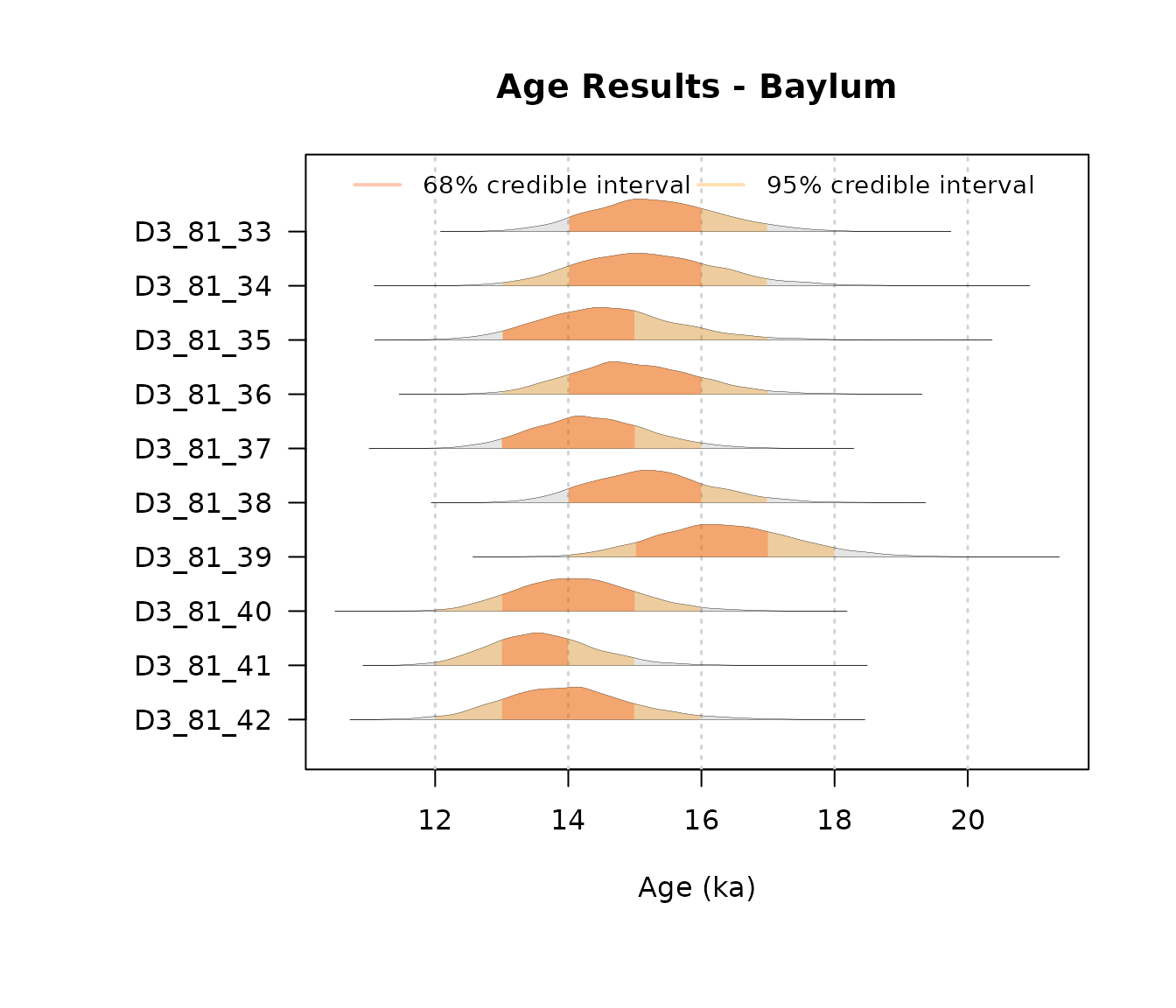

AgeWith_LogUniformOrder = plot_Ages(JingbianUO, plot_mode = "density")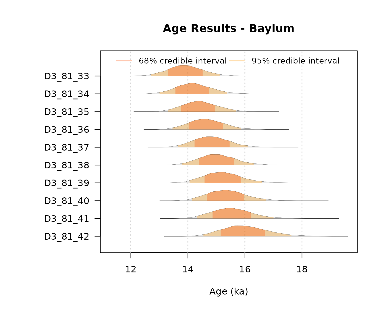

AgeWith_NJ = plot_Ages(JingbianNicholls, plot_mode = "density")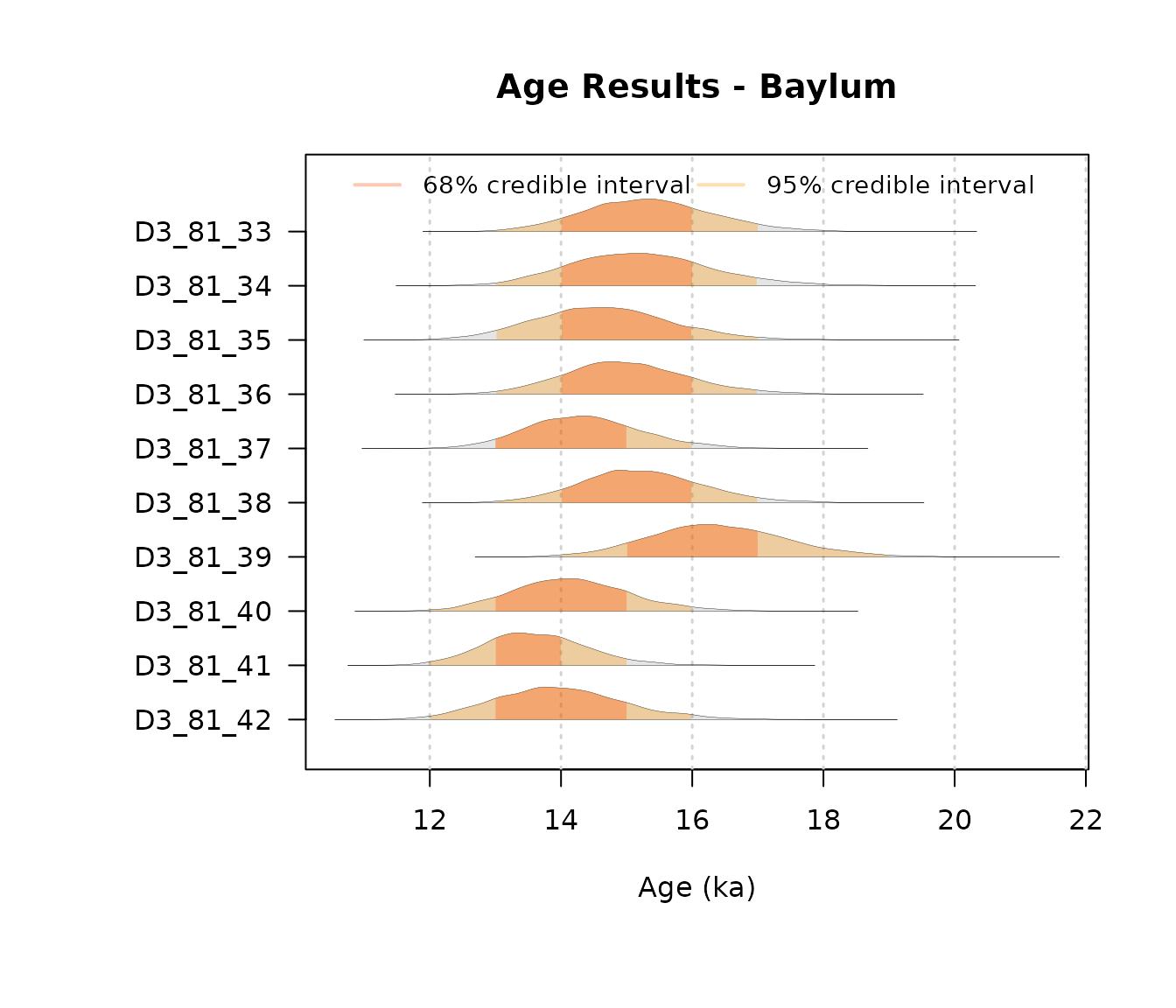

Graph Network and Stratigraphic Visualization

One can visualize the order links set up by the StratiConstraints matrix in a directed acyclic graph. The following code snippet provides the scheme on how to do that:

  # Create simple stratigraphic constraint matrix
create_mock_constraints <- function(n = 5) {
  
  matrix(c(rep(1, n), ## first row of ones
           c(0, 1, 1, 1, 1), rep(0, 5), 
           c(0,0, 0, 1, 1), c(rep(0, 4),1 ),
           rep(0, 5)),
         nrow = 6, byrow = TRUE)
}

reduced_network = remove_transitive_edges(create_mock_constraints()) 
# network visualization thanks to VisNetwork 
network_vizualization(reduced_network, interactive = T, vertices_labels = paste0("A", 1:5))

Isotonic Regression Computation

In this section, we introduce the function IsotonicCurve(), which computes the isotonic distortion of a posterior distribution obtained from the Compute_AgeS_D() function.

The currently supported priors for this isotonic correction are unconstrained priors.

This function requires the following arguments:

• StratiConstraints: The stratigraphic constraint matrix. This can either be provided directly or loaded from a file. If no matrix is supplied, the model assumes a strict chronological order.
• Object: The output object returned by the age model function Compute_AgeS_D().
• interactive: An optional argument. If not provided, the program will decide whether to display an interactive Directed Acyclic Graph (DAG) visualization in a web browser.
• level: Confidence levels for High Posterior Density (HPD) regions. The default values are 0.95 and 0.68.
• path: An optional path for saving the constraints DAG.

IsotonicDistorsion = IsotonicCurve(c(), OSLJingbian$Output,interactive = FALSE)

The function return a BayLum.list of three objects including the data.frame Ages:

knitr::kable(IsotonicDistorsion$Ages )

AGE	SD	MAP	SAMPLE	Unit	HPD68.MIN	HPD68.MAX	HPD95.MIN	HPD95.MAX
14.566	0.620	14.577	D3_81_33	1	13.930	15.158	13.332	15.788
14.625	0.601	14.923	D3_81_34	2	13.996	15.195	13.452	15.830
14.643	0.598	14.923	D3_81_35	3	14.027	15.215	13.473	15.839
14.671	0.594	15.328	D3_81_36	4	14.058	15.235	13.504	15.849
14.683	0.594	15.167	D3_81_37	5	14.067	15.244	13.518	15.863
14.727	0.595	14.278	D3_81_38	6	14.105	15.287	13.568	15.912
14.737	0.596	14.278	D3_81_39	7	14.115	15.297	13.568	15.922
14.737	0.596	14.278	D3_81_40	8	14.115	15.297	13.568	15.922
14.738	0.597	14.278	D3_81_41	9	14.115	15.297	13.568	15.922
14.826	0.655	14.355	D3_81_42	10	14.132	15.376	13.538	16.127

Similary to the compute_AgeS_D() function, the posterior marginals can be visualized with `plot_Ages()``

AgeWith_IR <-  plot_Ages(object = IsotonicDistorsion, plot_mode = "density")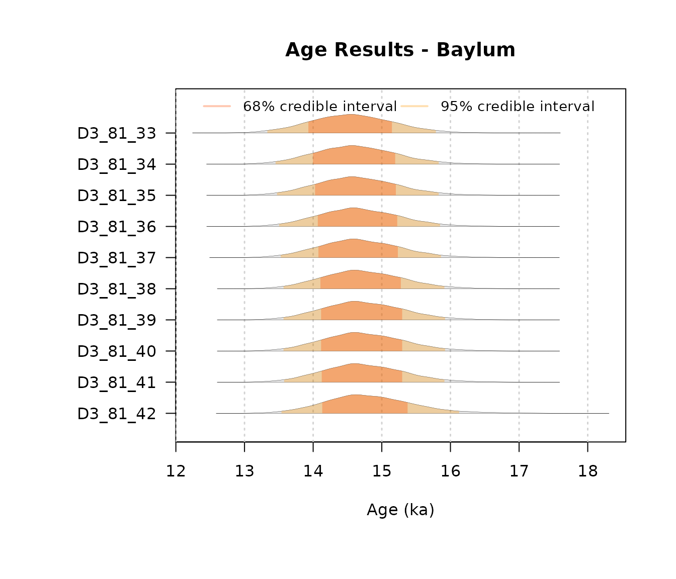

Note that the isotonic regression is computed following the Sequential Merging Block (SBM) algorithm presented in Wang et al. (2022).

To visualize the resulting posterior densities from the Isotonic Distorsion, we can use the function PlotIsotonicCurve() :

JingbianPlots = PlotIsotonicCurve(object = IsotonicDistorsion, level = .68)

The DAG constructed from the StratiConstraints matrix shows segments whose length represents the confidence interval (at the specified level) and gradient colors represent the age values for each sample. The y-axis has the same scale as the Bayesian mean estimators.

JingbianPlots$DAG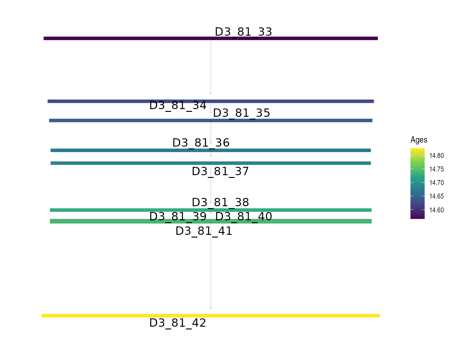

A ribbon plot showing the HPD regions of the distorted posterior distribution

JingbianPlots$ribbon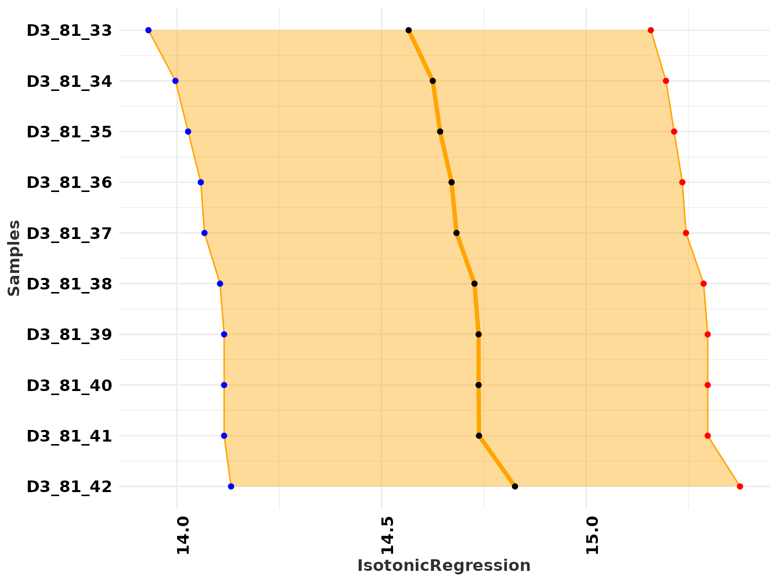

It is important to choose a level of HPD region / Credible interval already computed by IsotonicDistorsion() otherwise, the function return an error message.

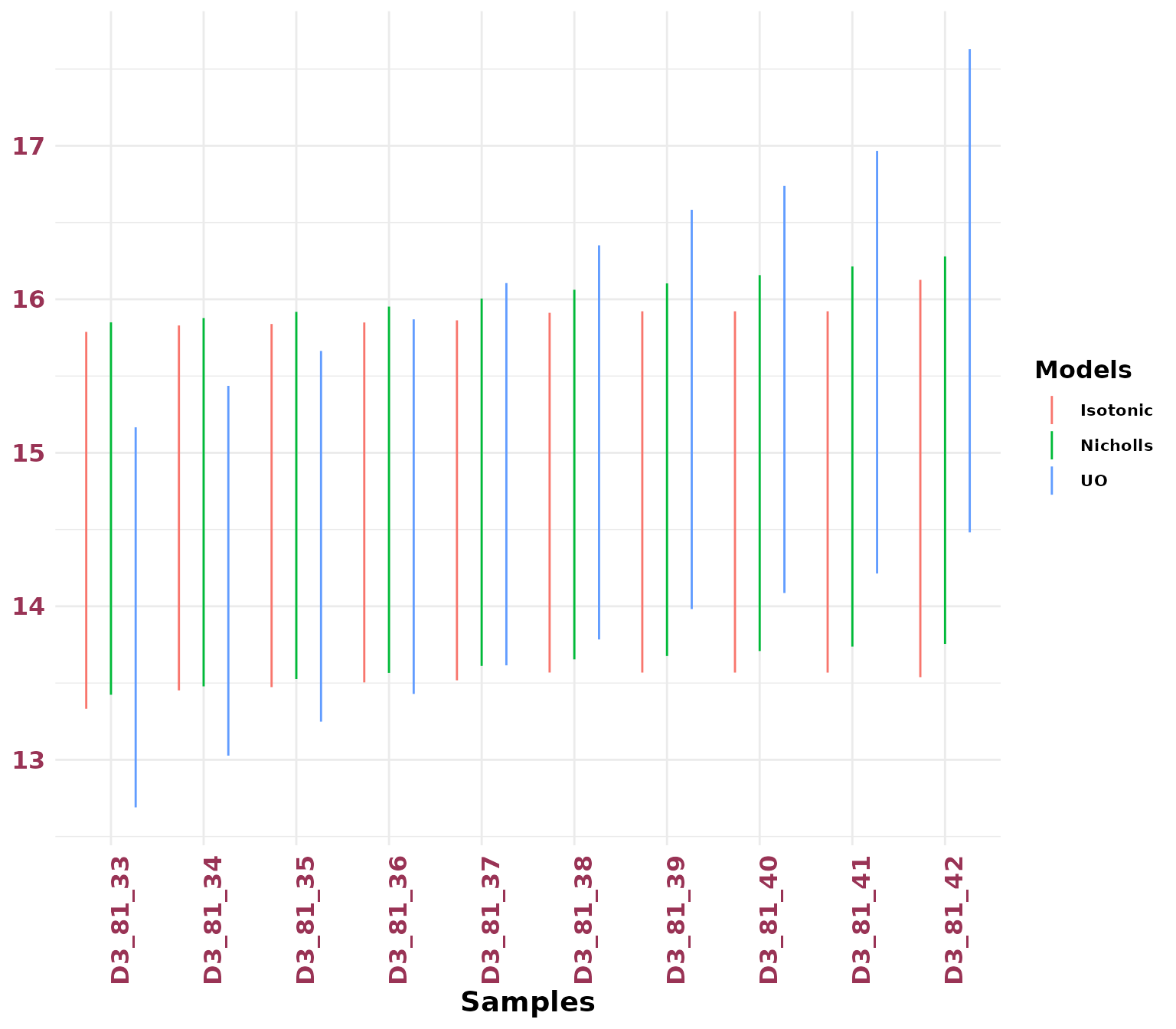
HPD Regions Plotting

We can compare multiple priors using the plotHpd() function. This function requires two main arguments:

• listObject: A list of output objects returned by Compute_AgeS_D() using different prior settings.
  
• Names: A character vector specifying the names for each age computation method, used to distinguish them in the plot.

plotHpd(list(JingbianUO, IsotonicDistorsion, JingbianNicholls), c("UO", "Isotonic", "Nicholls"))

References

Combès, Benoit, and Anne Philippe. 2017. “Bayesian Analysis of Individual and Systematic Multiplicative Errors for Estimating Ages with Stratigraphic Constraints in Optically Stimulated Luminescence Dating.” Quaternary Geochronology 39: 24–34.

Nicholls, Geoff K, and Peter W Jones. 2001. “Quantitative Archaeology and Bayesian Inference.” World Archaeology 33 (1): 92–109.

Wang, Xiwen, Jiaxi Ying, José Vinı́cius de M Cardoso, and Daniel P Palomar. 2022. “Efficient Algorithms for General Isotone Optimization.” In Proceedings of the AAAI Conference on Artificial Intelligence, 36:8575–83. 8.